Polydispersity & Orientational Distributions
For some models we can calculate the average intensity for a population of particles that possess size and/or orientational (ie, angular) distributions. In SasView we call the former polydispersity but use the parameter PD to parameterise both. In other words, the meaning of PD in a model depends on the actual parameter it is being applied too.
The resultant intensity is then normalized by the average particle volume such that
where \(F\) is the scattering amplitude and \(\langle\cdot\rangle\) denotes an average over the distribution \(f(x; \bar x, \sigma)\), giving
Each distribution is characterized by a center value \(\bar x\) or \(x_\text{med}\), a width parameter \(\sigma\) (note this is not necessarily the standard deviation, so read the description of the distribution carefully), the number of sigmas \(N_\sigma\) to include from the tails of the distribution, and the number of points used to compute the average. The center of the distribution is set by the value of the model parameter.
The distribution width applied to volume (ie, shape-describing) parameters is relative to the center value such that \(\sigma = \mathrm{PD} \cdot \bar x\). However, the distribution width applied to orientation parameters is just \(\sigma = \mathrm{PD}\).
\(N_\sigma\) determines how far into the tails to evaluate the distribution, with larger values of \(N_\sigma\) required for heavier tailed distributions. The scattering in general falls rapidly with \(qr\) so the usual assumption that \(f(r - 3\sigma_r)\) is tiny and therefore \(f(r - 3\sigma_r)f(r - 3\sigma_r)\) will not contribute much to the average may not hold when particles are large. This, too, will require increasing \(N_\sigma\).
Users should note that the averaging computation is very intensive. Applying polydispersion and/or orientational distributions to multiple parameters at the same time, or increasing the number of points in the distribution, will require patience! However, the calculations are generally more robust with more data points or more angles.
The following distribution functions are provided:
- Uniform Distribution
- Rectangular Distribution
- Gaussian Distribution
- Boltzmann Distribution
- Lognormal Distribution
- Schulz Distribution
- Array Distribution
These are all implemented as number-average distributions.
Additional distributions are under consideration.
Beware: when the Polydispersity & Orientational Distribution panel in SasView is first opened, the default distribution for all parameters is the Gaussian Distribution. This may not be suitable. See Suggested Applications below.
Note
In 2009 IUPAC decided to introduce the new term ‘dispersity’ to replace the term ‘polydispersity’ (see Pure Appl. Chem., (2009), 81(2), 351-353 in order to make the terminology describing distributions of chemical properties unambiguous. However, these terms are unrelated to the proportional size distributions and orientational distributions used in SasView models.
Suggested Applications
If applying polydispersion to parameters describing particle sizes, consider using the Lognormal or Schulz distributions.
If applying polydispersion to parameters describing interfacial thicknesses or angular orientations, consider using the Gaussian or Boltzmann distributions.
If applying polydispersion to parameters describing angles, use the Uniform distribution. Beware of using distributions that are always positive (eg, the Lognormal) because angles can be negative!
The array distribution allows a user-defined distribution to be applied.
Uniform Distribution
The Uniform Distribution is defined as
where \(\bar x\) (\(x_\text{mean}\) in the figure) is the mean of the distribution, \(\sigma\) is the half-width, and Norm is a normalization factor which is determined during the numerical calculation.
The polydispersity in sasmodels is given by

Fig. 127 Uniform distribution.
The value \(N_\sigma\) is ignored for this distribution.
Rectangular Distribution
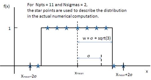
The Rectangular Distribution is defined as
where \(\bar x\) (\(x_\text{mean}\) in the figure) is the mean of the distribution, \(w\) is the half-width, and Norm is a normalization factor which is determined during the numerical calculation.
Note that the standard deviation and the half width \(w\) are different!
The standard deviation is
whilst the polydispersity in sasmodels is given by

Fig. 128 Rectangular distribution.
Note
The Rectangular Distribution is deprecated in favour of the Uniform Distribution above and is described here for backwards compatibility with earlier versions of SasView only.
Gaussian Distribution
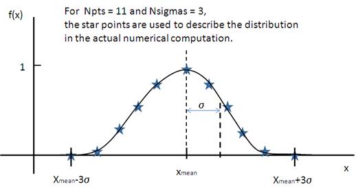
The Gaussian Distribution is defined as
where \(\bar x\) (\(x_\text{mean}\) in the figure) is the mean of the distribution and Norm is a normalization factor which is determined during the numerical calculation.
The polydispersity in sasmodels is given by

Fig. 129 Normal distribution.
Boltzmann Distribution
The Boltzmann Distribution is defined as
where \(\bar x\) (\(x_\text{mean}\) in the figure) is the mean of the distribution and Norm is a normalization factor which is determined during the numerical calculation.
The width is defined as
which is the inverse Boltzmann factor, where \(k\) is the Boltzmann constant, \(T\) the temperature in Kelvin and \(E\) a characteristic energy per particle.

Fig. 130 Boltzmann distribution.
Lognormal Distribution
The Lognormal Distribution describes a function of \(x\) where \(\ln (x)\) has a normal distribution. The result is a distribution that is skewed towards larger values of \(x\).
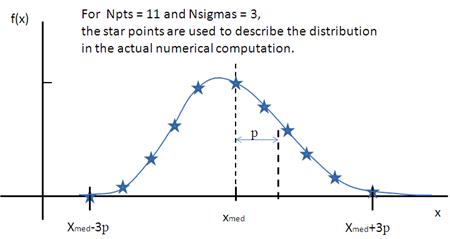
The Lognormal Distribution is defined as
where Norm is a normalization factor which will be determined during the numerical calculation, \(\mu=\ln(x_\text{med})\) and \(x_\text{med}\) is the median value of the lognormal distribution, but \(\sigma\) is a parameter describing the width of the underlying normal distribution.
\(x_\text{med}\) will be the value given for the respective size parameter in sasmodels, for example, radius=60.
The polydispersity in sasmodels is given by
The mean value of the distribution is given by \(\bar x = \exp(\mu+ \sigma^2/2)\) and the peak value by \(\max x = \exp(\mu - \sigma^2)\).
The variance (the square of the standard deviation) of the lognormal distribution is given by
Note that larger values of PD might need a larger number of points and \(N_\sigma\).

Fig. 131 Lognormal distribution for PD=0.1.
For further information on the Lognormal distribution see: http://en.wikipedia.org/wiki/Log-normal_distribution and http://mathworld.wolfram.com/LogNormalDistribution.html
Schulz Distribution
The Schulz (sometimes written Schultz) distribution is similar to the Lognormal distribution, in that it is also skewed towards larger values of \(x\), but which has computational advantages over the Lognormal distribution.
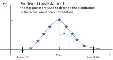
The Schulz distribution is defined as
where \(\bar x\) (\(x_\text{mean}\) in the figure) is the mean of the distribution, Norm is a normalization factor which is determined during the numerical calculation, and \(z\) is a measure of the width of the distribution such that
where \(p\) is the polydispersity in sasmodels given by
and \(\sigma\) is the RMS deviation from \(\bar x\).
Note that larger values of PD might need a larger number of points and \(N_\sigma\). For example, for PD=0.7 with radius=60 Å, at least Npts>=160 and Nsigmas>=15 are required.

Fig. 132 Schulz distribution.
For further information on the Schulz distribution see: M Kotlarchyk & S-H Chen, J Chem Phys, (1983), 79, 2461 and M Kotlarchyk, RB Stephens, and JS Huang, J Phys Chem, (1988), 92, 1533
Array Distribution
This user-definable distribution should be given as a simple ASCII text file where the array is defined by two columns of numbers: \(x\) and \(f(x)\). The \(f(x)\) will be normalized to 1 during the computation.
Example of what an array distribution file should look like:
| 30 | 0.1 |
| 32 | 0.3 |
| 35 | 0.4 |
| 36 | 0.5 |
| 37 | 0.6 |
| 39 | 0.7 |
| 41 | 0.9 |
Only these array values are used computation, therefore the parameter value given for the model will have no affect, and will be ignored when computing the average. This means that any parameter with an array distribution will not be fitable.
Note about DLS polydispersity
Several measures of polydispersity abound in Dynamic Light Scattering (DLS) and it should not be assumed that any of the following can be simply equated with the polydispersity PD parameter used in SasView.
The dimensionless Polydispersity Index (PI) is a measure of the width of the distribution of autocorrelation function decay rates (not the distribution of particle sizes itself, though the two are inversely related) and is defined by ISO 22412:2017 as
where \(\mu_\text{2}\) is the second cumulant, and \(\bar \Gamma^2\) is the intensity-weighted average value, of the distribution of decay rates.
If the distribution of decay rates is Gaussian then
where \(\sigma\) is the standard deviation, allowing a Relative Polydispersity (RP) to be defined as
PI values smaller than 0.05 indicate a highly monodisperse system. Values greater than 0.7 indicate significant polydispersity.
The size polydispersity P-parameter is defined as the relative standard deviation coefficient of variation
where \(\nu\) is the variance of the distribution and \(\bar R\) is the mean value of \(R\). Here, the product \(P \bar R\) is equal to the standard deviation of the Lognormal distribution.
P values smaller than 0.13 indicate a monodisperse system.
For more information see:
ISO 22412:2017, International Standards Organisation (2017).
Polydispersity: What does it mean for DLS and Chromatography.
Dynamic Light Scattering: Common Terms Defined, Whitepaper WP111214. Malvern Instruments (2011).
S King, C Washington & R Heenan, Phys Chem Chem Phys, (2005), 7, 143.
T Allen, in Particle Size Measurement, 4th Edition, Chapman & Hall, London (1990).
Document History