core_shell_bicelle_elliptical

Elliptical cylinder with a core-shell scattering length density profile..

Parameter	Description	Units	Default value
scale	Scale factor or Volume fraction	None	1
background	Source background	cm-1	0.001
radius	Cylinder core radius r_minor	Å	30
x_core	Axial ratio of core, X = r_major/r_minor	None	3
thick_rim	Rim shell thickness	Å	8
thick_face	Cylinder face thickness	Å	14
length	Cylinder length	Å	50
sld_core	Cylinder core scattering length density	10-6Å-2	4
sld_face	Cylinder face scattering length density	10-6Å-2	7
sld_rim	Cylinder rim scattering length density	10-6Å-2	1
sld_solvent	Solvent scattering length density	10-6Å-2	6
theta	Cylinder axis to beam angle	degree	90
phi	Rotation about beam	degree	0
psi	Rotation about cylinder axis	degree	0

The returned value is scaled to units of cm^-1 sr^-1, absolute scale.

Definition

This model provides the form factor for an elliptical cylinder with a core-shell scattering length density profile [1]. Thus this is a variation of the core-shell bicelle model, but with an elliptical cylinder for the core. Outer shells on the rims and flat ends may be of different thicknesses and scattering length densities. The form factor is normalized by the total particle volume.

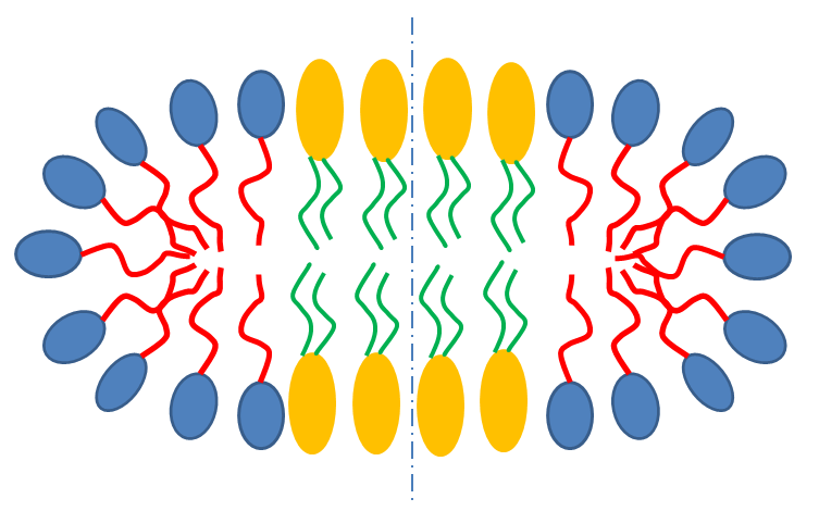
Fig. 11 Schematic cross-section of bicelle. Note however that the model here calculates for rectangular, not curved, rims as shown below.

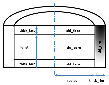
Fig. 12 Cross section of model used here. Users will have to decide how to distribute “heads” and “tails” between the rim, face and core regions in order to estimate appropriate starting parameters.

Given the scattering length densities (sld) \(\rho_c\), the core sld, \(\rho_f\), the face sld, \(\rho_r\), the rim sld and \(\rho_s\) the solvent sld, the scattering length density variation along the bicelle axis is:

\[\begin{split}\rho(r) = \begin{cases} &\rho_c \text{ for } 0 \lt r \lt R; -L \lt z\lt L \\[1.5ex] &\rho_f \text{ for } 0 \lt r \lt R; -(L+2t) \lt z\lt -L; L \lt z\lt (L+2t) \\[1.5ex] &\rho_r\text{ for } 0 \lt r \lt R; -(L+2t) \lt z\lt -L; L \lt z\lt (L+2t) \end{cases}\end{split}\]

The form factor for the bicelle is calculated in cylindrical coordinates, where \(\alpha\) is the angle between the \(Q\) vector and the cylinder axis, and \(\psi\) is the angle for the ellipsoidal cross section core, to give:

\[I(Q,\alpha,\psi) = \frac{\text{scale}}{V_t} \cdot F(Q,\alpha, \psi)^2 \cdot sin(\alpha) + \text{background}\]

where a numerical integration of \(F(Q,\alpha, \psi)^2 \cdot sin(\alpha)\) is carried out over alpha and psi for:

\begin{align*} F(Q,\alpha,\psi) = &\bigg[ (\rho_c - \rho_f) V_c \frac{2J_1(QR'sin \alpha)}{QR'sin\alpha} \frac{sin(QLcos\alpha/2)}{Q(L/2)cos\alpha} \\ &+(\rho_f - \rho_r) V_{c+f} \frac{2J_1(QR'sin\alpha)}{QR'sin\alpha} \frac{sin(Q(L/2+t_f)cos\alpha)}{Q(L/2+t_f)cos\alpha} \\ &+(\rho_r - \rho_s) V_t \frac{2J_1(Q(R'+t_r)sin\alpha)}{Q(R'+t_r)sin\alpha} \frac{sin(Q(L/2+t_f)cos\alpha)}{Q(L/2+t_f)cos\alpha} \bigg] \end{align*}

where

\[R'=\frac{R}{\sqrt{2}}\sqrt{(1+X_{core}^{2}) + (1-X_{core}^{2})cos(\psi)}\]

and \(V_t = \pi.(R+t_r)(Xcore.R+t_r)^2.(L+2.t_f)\) is the total volume of the bicelle, \(V_c = \pi.Xcore.R^2.L\) the volume of the core, \(V_{c+f} = \pi.Xcore.R^2.(L+2.t_f)\) the volume of the core plus the volume of the faces, \(R\) is the radius of the core, \(Xcore\) is the axial ratio of the core, \(L\) the length of the core, \(t_f\) the thickness of the face, \(t_r\) the thickness of the rim and \(J_1\) the usual first order bessel function. The core has radii \(R\) and \(Xcore.R\) so is circular, as for the core_shell_bicelle model, for \(Xcore\) =1. Note that you may need to limit the range of \(Xcore\), especially if using the Monte-Carlo algorithm, as setting radius to \(R/Xcore\) and axial ratio to \(1/Xcore\) gives an equivalent solution!

The output of the 1D scattering intensity function for randomly oriented bicelles is then given by integrating over all possible \(\alpha\) and \(\psi\).

For oriented bicelles the theta, phi and psi orientation parameters will appear when fitting 2D data, see the elliptical_cylinder model for further information.

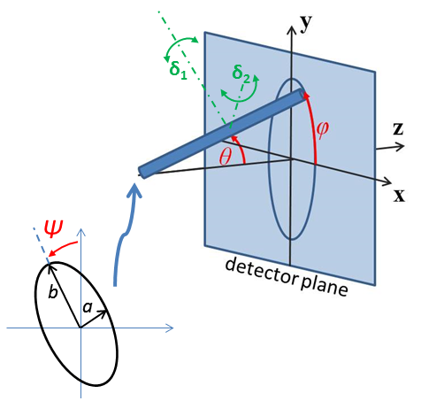
Fig. 13 Definition of the angles for the oriented core_shell_bicelle_elliptical particles.

Model verified using Monte Carlo simulation for 1D and 2D scattering.

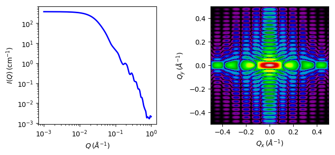
Fig. 14 1D and 2D plots corresponding to the default parameters of the model.

Source

core_shell_bicelle_elliptical.py \(\ \star\ \) core_shell_bicelle_elliptical.c \(\ \star\ \) lib/gauss76.c \(\ \star\ \) lib/sas_J1.c \(\ \star\ \) lib/polevl.c \(\ \star\ \) lib/sas_Si.c

References

[1]	Onsager, Ann. New York Acad. Sci., 51 (1949) 627-659

Authorship and Verification

• Author: Richard Heenan Date: December 14, 2016
• Last Modified by: Richard Heenan Date: December 14, 2016
• Last Reviewed by: Paul Kienzle Date: Feb 28, 2018