Polydispersity & Orientational Distributions
For some models we can calculate the average intensity for a population of particles that possess size and/or orientational (ie, angular) distributions (see Theory for more details). In SasView we call the former polydispersity but use the parameter PD to parameterise both. In other words, the meaning of PD in a model depends on the actual parameter it is being applied too.
The resultant intensity is then normalized by the average particle volume such that
where \(F\) is the scattering amplitude and \(\langle\cdot\rangle\) denotes an average over the distribution \(f(x; \bar x, \sigma)\), giving
Each distribution is characterized by a center value \(\bar x\) or \(x_\text{med}\), a width parameter \(\sigma\) (note this is not necessarily the standard deviation, so read the description carefully), the number of sigmas \(N_\sigma\) to include from the tails of the distribution, and the number of points used to compute the average. The center of the distribution is set by the value of the model parameter. The meaning of a polydispersity parameter PD (not to be confused with a molecular weight distributions in polymer science) in a model depends on the type of parameter it is being applied too.
The distribution width applied to volume (ie, shape-describing) parameters is relative to the center value such that \(\sigma = \mathrm{PD} \cdot \bar x\). However, the distribution width applied to orientation (ie, angle-describing) parameters is just \(\sigma = \mathrm{PD}\).
\(N_\sigma\) determines how far into the tails to evaluate the distribution, with larger values of \(N_\sigma\) required for heavier tailed distributions. The scattering in general falls rapidly with \(qr\) so the usual assumption that \(f(r - 3\sigma_r)\) is tiny and therefore \(f(r - 3\sigma_r)f(r - 3\sigma_r)\) will not contribute much to the average may not hold when particles are large. This, too, will require increasing \(N_\sigma\).
Users should note that the averaging computation is very intensive. Applying polydispersion and/or orientational distributions to multiple parameters at the same time, or increasing the number of points in the distribution, will require patience! However, the calculations are generally more robust with more data points or more angles.
The following distribution functions are provided:
These distributions define the number density of the given population of scatterers. The resulting scattering is then the number average over the distribution.
Beware: the default distribution for all parameters is the Gaussian Distribution but this may not be suitable. See Suggested Applications below.
Note
In 2009 IUPAC decided to introduce the new term ‘dispersity’ to replace the term ‘polydispersity’ (see Pure Appl. Chem., (2009), 81(2), 351-353 in order to make the terminology describing distributions of chemical properties unambiguous. However, these terms are unrelated to the proportional size distributions and orientational distributions used in SasView models.
Suggested Applications
If applying polydispersion to parameters describing particle sizes, consider using the Lognormal Distribution or Schulz Distribution.
If applying polydispersion to parameters describing interfacial thicknesses or orientations, consider using the Gaussian Distribution or Boltzmann Distribution.
If applying polydispersion to parameters describing angles, use the Uniform Distribution or a Maier-Saupe distribution or a Cyclic Gaussian distribution.
The Array Distribution provides a very simple means of implementing a user-defined distribution, but without any fittable parameters. Greater flexibility is conferred by using User-defined Distributions.
Usage Notes
Beware of using distributions that are always positive (eg, the Lognormal) for angles because angles can be negative! If in doubt, plot the polydispersity data for the model and check!
The parameter bounds (ie, Min/Max) for polydispersion should be specified under the Polydispersity tab on the FitPage. They are not formally linked to the bounds for the parameter to which polydispersion is being applied that appear under the Model tab. In other words, bounds on a radius parameter under Model are not the same as bounds on a distribution of radius parameter under Polydispersity, and vice versa.
If a distribution exceeds its parameter bounds those weights outside the bounds are excluded and the distribution is normalized such that the sum of the remaining weights in the truncated distribution equal one.
Whilst PD values for ‘size’ parameters are in proportion to the mean, with values normally lying in the range 0 – 1, PD values for ‘angular’ parameters represent the actual width of the distribution in degrees, so values as high as 5 or 10 degrees maybe necessary to describe oriented systems. Again, plotting the relevant polydispersity data will easily show if a sensible value is being used.
When using an Array Distribution, be aware that the polydispersity parameters, and the parameter to which the distribution is being applied, cannot be fitted.
Additional distribution functions (and, indeed models) may be found on the Sasview Model Marketplace.
Uniform Distribution
The Uniform Distribution is defined as
where \(\bar x\) (\(x_\text{mean}\) in the figure) is the mean of the distribution, \(\sigma\) is the half-width, and Norm is a normalization factor which is determined during the numerical calculation.
The polydispersity in sasmodels is given by
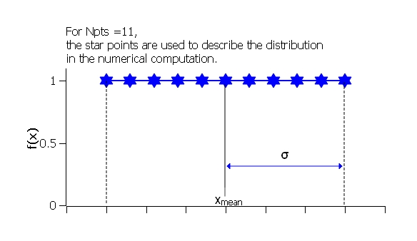
Fig. 130 Uniform distribution.
The value \(N_\sigma\) is ignored for this distribution.
Rectangular Distribution
The Rectangular Distribution is defined as
where \(\bar x\) (\(x_\text{mean}\) in the figure) is the mean of the distribution, \(w\) is the half-width, and Norm is a normalization factor which is determined during the numerical calculation.
Note that the standard deviation and the half width \(w\) are different!
The standard deviation is
whilst the polydispersity in sasmodels is given by
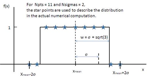
Fig. 131 Rectangular distribution.
Note
The Rectangular Distribution is deprecated in favour of the Uniform Distribution above and is described here for backwards compatibility with earlier versions of SasView only.
Gaussian Distribution
The Gaussian Distribution is defined as
where \(\bar x\) (\(x_\text{mean}\) in the figure) is the mean of the distribution and Norm is a normalization factor which is determined during the numerical calculation.
The polydispersity in sasmodels is given by
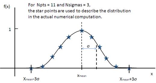
Fig. 132 Normal distribution.
Boltzmann Distribution
The Boltzmann Distribution is defined here as
where \(\bar x\) (\(x_\text{mean}\) in the figure) is the mean of the distribution and Norm is a normalization factor which is determined during the numerical calculation. Strictly speaking, however, this function is a Laplace Distribution, of which the Boltzmann Distribution is but a limiting case.
The width is defined as
which is the inverse Boltzmann factor, where \(k\) is the Boltzmann constant, \(T\) the temperature in Kelvin and \(E\) a characteristic energy per particle.
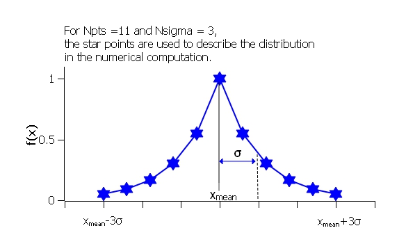
Fig. 133 Boltzmann distribution.
Lognormal Distribution
The Lognormal Distribution describes a function of \(x\) where \(\ln (x)\) has a normal distribution. The result is a distribution that is skewed towards larger values of \(x\).
The Lognormal Distribution is defined as
where Norm is a normalization factor which will be determined during the numerical calculation, \(\mu=\ln(x_\text{med})\) and \(x_\text{med}\) is the median value of the lognormal distribution, but \(\sigma\) is a parameter describing the width of the underlying normal distribution.
\(x_\text{med}\) will be the value given for the respective size parameter in sasmodels, for example, radius=60.
The polydispersity in sasmodels is given by
The mean value of the distribution is given by \(\bar x = \exp(\mu+ \sigma^2/2)\) and the peak value by \(\max x = \exp(\mu - \sigma^2)\).
The variance (the square of the standard deviation) of the lognormal distribution is given by
Note that larger values of PD might need a larger number of points and \(N_\sigma\).
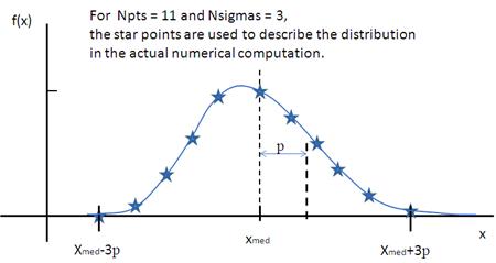
Fig. 134 Lognormal distribution for PD=0.1.
For further information on the Lognormal distribution see:
Schulz Distribution
The Schulz (sometimes written Schultz) distribution is similar to the Lognormal distribution, in that it is also skewed towards larger values of \(x\), but which has computational advantages over the Lognormal distribution.
The Schulz distribution is defined as
where \(\bar x\) (\(x_\text{mean}\) in the figure) is the mean of the distribution, Norm is a normalization factor which is determined during the numerical calculation, and \(z\) is a measure of the width of the distribution such that
where \(p\) is the polydispersity in sasmodels given by
and \(\sigma\) is the RMS deviation from \(\bar x\).
Note that larger values of PD might need a larger number of points and \(N_\sigma\). For example, for PD=0.7 with radius=60 Å, at least Npts>=160 and Nsigmas>=15 are required.
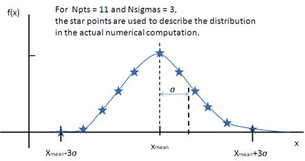
Fig. 135 Schulz distribution.
For further information on the Schulz distribution see:
M Kotlarchyk & S-H Chen, J Chem Phys, (1983), 79, 2461
M Kotlarchyk, RB Stephens, and JS Huang, J Phys Chem, (1988), 92, 1533.
Array Distribution
This user-definable distribution should be given as a simple ASCII text file where the array is defined by two columns of numbers: \(x\) and \(f(x)\). The \(f(x)\) will be normalized to 1 during the computation.
Example of what an array distribution file should look like:
30 |
0.1 |
32 |
0.3 |
35 |
0.4 |
36 |
0.5 |
37 |
0.6 |
39 |
0.7 |
41 |
0.9 |
Note
Only these array values are used for computation, any other polydispersity parameter values in the model have no effect and will be ignored when computing the average. This also means that any parameter with an array distribution cannot be fitted.
If representing continuous distributions, it is best to use a simple rectangle rule integration with equally spaced \(x\) values and the weight \(f(x)\) chosen at the center of each interval.
User-defined Distributions
You can also define your own distribution by creating a python file defining a Distribution object with a _weights method. The _weights method takes center, sigma, lb and ub as arguments, and can access self.npts and self.nsigmas from the distribution. They are interpreted as follows:
center the value of the shape parameter (for size dispersity) or zero if it is an angular dispersity. This parameter may be fitted.
sigma the width of the distribution, which is the polydispersity parameter times the center for size dispersity, or the polydispersity parameter alone for angular dispersity. This parameter may be fitted.
lb, ub are the parameter limits (lower & upper bounds) given in the model definition file. For example, a radius parameter has lb equal to zero. A volume fraction parameter would have lb equal to zero and ub equal to one.
self.nsigmas the distance to go into the tails when evaluating the distribution. For a two parameter distribution, this value could be co-opted to use for the second parameter, though it will not be available for fitting.
self.npts the number of points to use when evaluating the distribution. The user will adjust this to trade calculation time for accuracy, but the distribution code is free to return more or fewer, or use it for the third parameter in a three parameter distribution.
As an example, the code following wraps the Laplace distribution from scipy stats:
import numpy as np
from scipy.stats import laplace

from sasmodels import weights

class Dispersion(weights.Dispersion):
    r"""
    Laplace distribution

    .. math::

        w(x) = e^{-\sigma |x - \mu|}
    """
    type = "laplace"
    default = dict(npts=35, width=0, nsigmas=3)  # default values
    def _weights(self, center, sigma, lb, ub):
        x = self._linspace(center, sigma, lb, ub)
        wx = laplace.pdf(x, center, sigma)
        return x, wx
You can plot the weights for a given value and width using the following:
from numpy import inf
from matplotlib import pyplot as plt
from sasmodels import weights

# reload the user-defined weights
weights.load_weights()
x, wx = weights.get_weights('laplace', n=35, width=0.1, nsigmas=3, value=50,
                            limits=[0, inf], relative=True)

# plot the weights
plt.interactive(True)
plt.plot(x, wx, 'x')
The self.nsigmas and self.npts parameters are normally used to control the accuracy of the distribution integral. The self._linspace function uses them to define the x values (along with the center, sigma, lb, and ub which are passed as parameters). If you repurpose npts or nsigmas you will need to generate your own x. Be sure to honour the limits lb and ub, for example to disallow a negative radius or constrain the volume fraction to lie between zero and one.
To activate a user-defined distribution, put it in a file such as distname.py in the SAS_WEIGHTS_PATH folder. This is defined with an environment variable, defaulting to:
SAS_WEIGHTS_PATH=~/.sasview/weights
or on Windows:
SAS_WEIGHTS_PATH=%USERPROFILE%\.sasview\weights
The weights path is loaded on startup. To update the distribution definition in a running application you will need to enter the following python commands:
import sasmodels.weights
sasmodels.weights.load_weights('path/to/distname.py')
Note about DLS polydispersity
Several measures of polydispersity abound in Dynamic Light Scattering (DLS) and it should not be assumed that any of the following can be simply equated with the polydispersity PD parameter used in SasView.
The dimensionless Polydispersity Index (PI) is a measure of the width of the distribution of autocorrelation function decay rates (not the distribution of particle sizes itself, though the two are inversely related) and is defined by ISO 22412:2017 as
where \(\mu_\text{2}\) is the second cumulant, and \(\bar \Gamma^2\) is the intensity-weighted average value, of the distribution of decay rates.
If the distribution of decay rates is Gaussian then
where \(\sigma\) is the standard deviation, allowing a Relative Polydispersity (RP) to be defined as
PI values smaller than 0.05 indicate a highly monodisperse system. Values greater than 0.7 indicate significant polydispersity.
The size polydispersity P-parameter is defined as the relative standard deviation coefficient of variation
where \(\nu\) is the variance of the distribution and \(\bar R\) is the mean value of \(R\). Here, the product \(P \bar R\) is equal to the standard deviation of the Lognormal distribution.
P values smaller than 0.13 indicate a monodisperse system.
For more information see:
ISO 22412:2017, International Standards Organisation (2017).
Polydispersity: What does it mean for DLS and Chromatography.
Dynamic Light Scattering: Common Terms Defined, Whitepaper WP111214. Malvern Instruments (2011).
S King, C Washington & R Heenan, Phys Chem Chem Phys, (2005), 7, 143.
T Allen, in Particle Size Measurement, 4th Edition, Chapman & Hall, London (1990).
Document History