broad_peak

Broad Lorentzian type peak on top of a power law decay

Parameter	Description	Units	Default value
scale	Scale factor or Volume fraction	None	1
background	Source background	cm-1	0.001
porod_scale	Power law scale factor	None	1e-05
porod_exp	Exponent of power law	None	3
lorentz_scale	Scale factor for broad Lorentzian peak	None	10
lorentz_length	Lorentzian screening length	Å	50
peak_pos	Peak position in q	Å-1	0.1
lorentz_exp	Exponent of Lorentz function	None	2

The returned value is scaled to units of cm^-1 sr^-1, absolute scale.

Definition

This model calculates an empirical functional form for SAS data characterized by a broad scattering peak. Many SAS spectra are characterized by a broad peak even though they are from amorphous soft materials. For example, soft systems that show a SAS peak include copolymers, polyelectrolytes, multiphase systems, layered structures, etc.

The d-spacing corresponding to the broad peak is a characteristic distance between the scattering inhomogeneities (such as in lamellar, cylindrical, or spherical morphologies, or for bicontinuous structures).

The scattering intensity $I(q)$ is calculated as

$$I(q) = \frac{A}{q^n} + \frac{C}{1 + (|q - q_0|\xi)^m} + B$$

Here the peak position is related to the d-spacing as $q_0 = 2\pi / d_0$.

$A$ is the Porod law scale factor, $n$ the Porod exponent, $C$ is the Lorentzian scale factor, $m$ the exponent of $q$, $\xi$ the screening length, and $B$ the flat background.

For 2D data the scattering intensity is calculated in the same way as 1D, where the $q$ vector is defined as

$$q = \sqrt{q_x^2 + q_y^2}$$

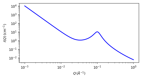
Fig. 99 1D plot corresponding to the default parameters of the model.

Source

broad_peak.py

References

None.

Authorship and Verification

• Author: NIST IGOR/DANSE Date: pre 2010

• Last Modified by: Paul kienle Date: July 24, 2016

• Last Reviewed by: Richard Heenan Date: March 21, 2016