porod
Porod function
Parameter |
Description |
Units |
Default value |
|---|---|---|---|
scale |
Scale factor or Volume fraction |
None |
1 |
background |
Source background |
cm-1 |
0.001 |
The returned value is scaled to units of cm-1 sr-1, absolute scale.
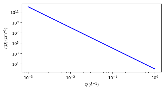
This model is a special case of the power law model, deriving its special name from the Porod Law which it models, where the power law exponent is fixed to -4.
Where the power law constant C in this case is just the scale factor.
The Porod law, similar to the Guinier model, is a broadly applicable model to a very restricted portion of the data. While the Guinier model applies to any dilute particulate system regardless of shape or size but only to the very low q (being a taylor expansion around q = 0), the Porod Law applies to any scattering system with sharp scattering length density interfaces between the phases but only at very high q (technically in the limit as q→∞ .. except of course that, practically, the continuum approach breaks down there). It is based on the idea that at sufficiently high q there is no shape information left and all scattering is just reflections off the sharp interfaces.
In the special case of a two phase system, the power law constant C derived from the appropriate q limit portion of the data is known as the Porod Constant and can be written as:
where Sv is the specific surface area (ie, surface area / volume) of the material under study, and Δρ is the contrast factor between the two phases.
Thus, by extracting the Porod Constant from experimental data, and knowing the contrast factor between the two phases, one can obtain the specific surface area for the material. This can be very useful for example in understanding porosity in materials, particularly when used in conjunction with complementary techniques such as BET.
Note
While it is straightforward to calculate the specific surface area, Sv of the material from the Porod Constant returned here, the Invariant analysis panel will also compute the Sv by entering the contrast term and the Porod Constant obtained here into the appropriate entry boxes.
There are, however, several caveats regarding obtaining a good experimental value of the Porod Constant.
First, as it is the scale value, the data must be on an absolute scale.
Next of course, there must be a sufficiently large q range that is in the Porod region to be able to be fit. But this may not always be possible: for example, polymer coils in solution will often not reach that limit within typical SAS ranges, nor even the q ranges where the continuum approach of using the SLD is even valid.
For highly monodisperse systems with limited resolution smearing, the data will contain large oscillations which will make the estimate from this fit unreliable. It will vary depending on the exact range of the fit that is chosen. This is because numerical integration using a finite number of points cannot properly capture the exact area under the data across these very sharp dips.
Ironically, large resolution smearing, and/or polydispersity smearing, will make the value obtained much more consistent and reliable. Thus the problem is less severe for typical real data than for simulated data that does not simulate any resolution smearing.
If in any doubt, using several values of qmin in the fitting, and comparing with the value obtained in a different manner, is highly advisable. One such method uses the Porod plot (I(q)∗q4 vs. q4). Fitting the highest q (strictly speaking q4) data to a straight line using as much of the high q as fits well to a straight line, yields a slope which is the flat background and an intercept which is the Porod Constant.
For 2D data: The 2D scattering intensity is calculated in the same way as 1D, where the q vector is defined as

Fig. 117 1D plot corresponding to the default parameters of the model.
Source
References
G Porod. Kolloid Zeit. 124 (1951) 83
L A Feigin, D I Svergun, G W Taylor. Structure Analysis by Small-Angle X-ray and Neutron Scattering. Springer. (1987)
Authorship and Verification
Author:
Last Modified by: Paul Butler, 28Mar2020
Last Reviewed by: