two_power_law

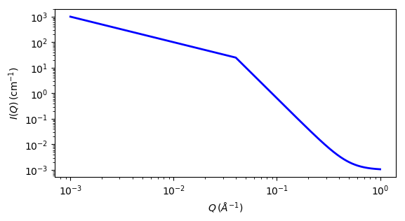
This model calculates an empirical functional form for SAS data characterized by two power laws.

Parameter	Description	Units	Default value
scale	Scale factor or Volume fraction	None	1
background	Source background	cm-1	0.001
coefficent_1	coefficent A in low Q region	None	1
crossover	crossover location	Å-1	0.04
power_1	power law exponent at low Q	None	1
power_2	power law exponent at high Q	None	4

The returned value is scaled to units of cm^-1 sr^-1, absolute scale.

Definition

The scattering intensity $I(q)$ is calculated as

$$\begin{split}I(q) = \begin{cases} A q^{-m1} + \text{background} & q <= q_c \\ C q^{-m2} + \text{background} & q > q_c \end{cases}\end{split}$$

where $q_c$ = the location of the crossover from one slope to the other, $A$ = the scaling coefficient that sets the overall intensity of the lower Q power law region, $m1$ = power law exponent at low Q, and $m2$ = power law exponent at high Q. The scaling of the second power law region (coefficient C) is then automatically scaled to match the first by following formula:

$$C = \frac{A q_c^{m2}}{q_c^{m1}}$$

Note

Be sure to enter the power law exponents as positive values!

For 2D data the scattering intensity is calculated in the same way as 1D, where the $q$ vector is defined as

$$q = \sqrt{q_x^2 + q_y^2}$$

Fig. 125 1D plot corresponding to the default parameters of the model.

Source

two_power_law.py

References

None.

Authorship and Verification

• Author: NIST IGOR/DANSE Date: pre 2010

• Last Modified by: Wojciech Wpotrzebowski Date: February 18, 2016

• Last Reviewed by: Paul Butler Date: March 21, 2016