Oriented Particles
With two dimensional small angle diffraction data sasmodels will calculate scattering from oriented particles, applicable for example to shear flow or orientation in a magnetic field.
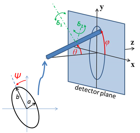
In general we first need to define the reference orientation of the particle’s a-b-c axes with respect to the incoming neutron or X-ray beam. This is done using three angles: θ and ϕ define the orientation of the c-axis of the particle, and angle Ψ is defined as the orientation of the major axis of the particle cross section with respect to its starting position along the beam direction (or equivalently, as rotation about the c axis). There is an unavoidable ambiguity when c is aligned with z in that ϕ and Ψ both serve to rotate the particle about c, but this symmetry is destroyed when θ is not a multiple of 180.
The figures below are for an elliptical cross section cylinder, but may be applied analogously to other shapes of particle.
Note
It is very important to note that these angles, in particular θ and ϕ, are NOT in general the same as the θ and ϕ appearing in equations for the scattering form factor which gives the scattered intensity or indeed in the equation for scattering vector Q. The θ rotation must be applied before the ϕ rotation, else there is an ambiguity.

Fig. 137 Definition of angles for oriented elliptical cylinder, where axis_ratio b/a is shown >1. Note that rotation θ, initially in the x-z plane, is carried out first, then rotation ϕ about the z-axis, finally rotation Ψ is around the axis of the cylinder. The neutron or X-ray beam is along the −z axis.

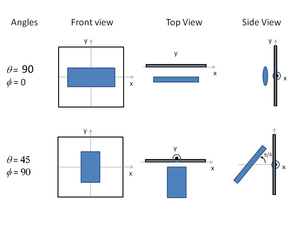
Fig. 138 Some examples of the orientation angles for an elliptical cylinder, with Ψ = 0.
Having established the mean direction of the particle (the view) we can then apply angular orientation distributions (jitter). This is done by a numerical integration over a range of angles in a similar way to particle size dispersity. The orientation dispersity is defined with respect to the a-b-c axes of the particle, with roll angle Ψ about the c-axis, yaw angle θ about the b-axis and pitch angle ϕ about the a-axis.
You can explore the view and jitter angles interactively using
sasmodels.jitter.run(). Enter the following into the python
interpreter:
from sasmodels import jitter
jitter.run()
More formally, starting with axes a-b-c of the particle aligned with axes x-y-z of the laboratory frame, the orientation dispersity is applied first, using the Tait-Bryan x-y′-z″ convention with angles \Delta\phi-\Delta\theta-\Delta\Psi. The reference orientation then follows, using the Euler angles z-y'-z'' with angles \phi-\theta-\Psi. This is implemented using rotation matrices as
To transform detector (q_x, q_y) values into (q_a, q_b, q_c) for the shape in its canonical orientation, use
The inverse rotation is easily calculated by rotating the opposite directions in the reverse order, so
The \theta and \phi orientation parameters for the cylinder only appear when fitting 2d data. On introducing “Orientational Distribution” in the angles, “distribution of theta” and “distribution of phi” parameters will appear. These are actually rotations about the axes \delta_1 and \delta_2 of the cylinder, which correspond to the b and a axes of the cylinder cross section. (When \theta = \phi = 0 these are parallel to the Y and X axes of the instrument.) The third orientation distribution, in \Psi, is about the c axis of the particle. Some experimentation may be required to understand the 2d patterns fully. A number of different shapes of distribution are available, as described for size dispersity, see Polydispersity & Orientational Distributions.
Given that the angular dispersion distribution is defined in cartesian space, over a cube defined by
but the orientation is defined over a sphere, we are left with a map projection problem, with different tradeoffs depending on how values in \Delta\theta and \Delta\phi are translated into latitude/longitude on the sphere.
Sasmodels is using the equirectangular projection. In this projection, square patches in angular dispersity become wedge-shaped patches on the sphere. To correct for the changing point density, there is a scale factor of \sin(\Delta\theta) that applies to each point in the integral. This is not enough, though. Consider a shape which is tumbling freely around the b axis, with \Delta\theta uniform in [-180, 180]. At \pm 90, all points in \Delta\phi map to the pole, so the jitter will have a distinct angular preference. If the spin axis is along the beam (which will be the case for \theta=90 and \Psi=90) the scattering pattern should be circularly symmetric, but it will go to zero at q_x = 0 due to the \sin(\Delta\theta) correction. This problem does not appear for a shape that is tumbling freely around the a axis, with \Delta\phi uniform in [-180, 180], so swap the a and b axes so \Delta\theta < \Delta\phi and adjust \Psi by 90. This works with the current sasmodels shapes due to symmetry.
Alternative projections were considered. The sinusoidal projection works by scaling \Delta\phi as \Delta\theta increases, and dropping those points outside [-180, 180]. The distortions are a little less for middle ranges of \Delta\theta, but they are still severe for large \Delta\theta and the model is much harder to explain. The azimuthal equidistance projection also improves on the equirectangular projection by extending the range of reasonable values for the \Delta\theta range, with \Delta\phi forming a wedge that cuts to the opposite side of the sphere rather than cutting to the pole. This projection has the nice property that distance from the center are preserved, and that \Delta\theta and \Delta\phi act the same. The azimuthal equal area projection is like the azimuthal equidistance projection, but it preserves area instead of distance. It also has the same behaviour for \Delta\theta and \Delta\phi. The Guyou projection has an excellent balance with reasonable distortion in both \Delta\theta and \Delta\phi, as well as preserving small patches. However, it requires considerably more computational overhead, and we have not yet derived the formula for the distortion correction, measuring the degree of stretch at the point (\Delta\theta, \Delta\phi) on the map.
Note
Note that the form factors for oriented particles are performing numerical integrations over one or more variables, so care should be taken, especially with very large particles or more extreme aspect ratios. In such cases results may not be accurate, particularly at very high Q, unless the model has been specifically coded to use limiting forms of the scattering equations.
For best numerical results keep the \theta distribution narrower than the \phi distribution. Thus for asymmetric particles, such as elliptical_cylinder, you may need to reorder the sizes of the three axes to acheive the desired result. This is due to the issues of mapping a rectanglar distribution onto the surface of a sphere.
Users can experiment with the values of Npts and Nsigs, the number of steps used in the integration and the range spanned in number of standard deviations. The standard deviation is entered in units of degrees. For a “rectangular” distribution the full width should be \pm \sqrt(3) ~ 1.73 standard deviations. The new “uniform” distribution avoids this by letting you directly specify the half width.
The angular distributions may be truncated outside of the range -180 to +180 degrees, so beware of using saying a broad Gaussian distribution with large value of Nsigs, as the array of Npts may be truncated to many fewer points than would give a good integration,as well as becoming rather meaningless. (At some point in the future the actual dispersion arrays may be made available to the user for inspection.)
Some more detailed technical notes are provided in the developer section of this manual Orientation and Numerical Integration .
This definition of orientation is new to SasView 4.2. In earlier versions, the orientation distribution appeared as a distribution of view angles. This led to strange effects when c was aligned with z, where changes to the \phi angle served only to rotate the shape about c, rather than having a consistent interpretation as the pitch of the shape relative to the flow field defining the reference orientation. Prior to SasView 4.1, the reference orientation was defined using a Tait-Bryan convention, making it difficult to control. Now, rotation in \theta modifies the spacings in the refraction pattern, and rotation in \phi rotates it in the detector plane.