How To Use Corfunc
Running a Calculation
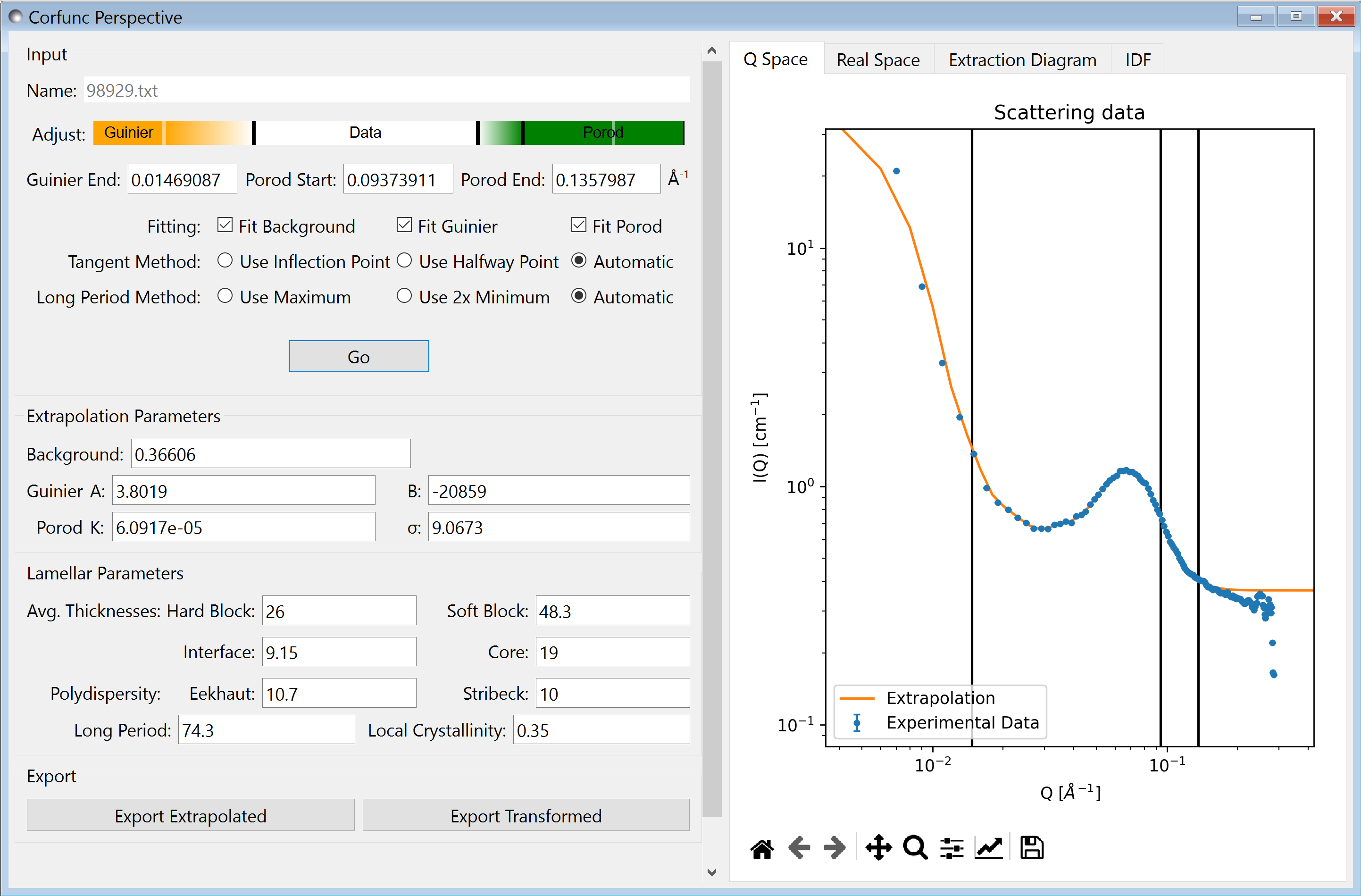
Upon sending data for correlation function analysis, it will be plotted (minus the background value), along with a bar indicating the upper end of the low-Q range (used for Guinier back-extrapolation) and 2 bars indicating the range to be used for Porod forward-extrapolation.
This information is also shown on the orange and green interactive slider on the left. You can drag bars on this slider (not the plot), or enter values manually.
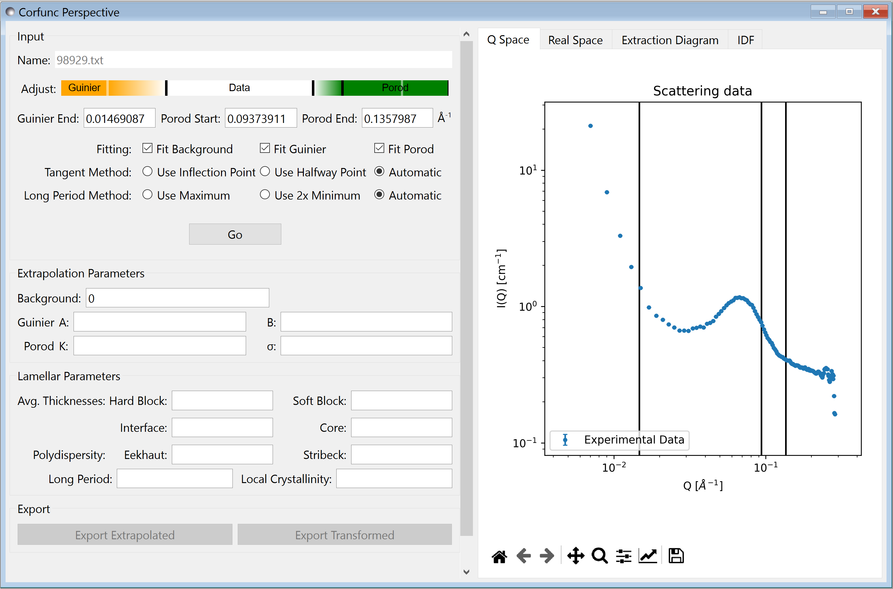
Once the Q ranges have been set, click the “Go” button to run the analysis. This will run through the process described in the technical documentation using the default options shown above the button.
The parameters used along the way can be overriden by changing them in the appropriate text boxes, and whether or not they are recalculated is controlled by the check boxes.
Options
In addition to the checkboxes that control whether parts of the calculation are executed, there are options for choosing how the lamellar parameters are extracted. These are intended to give flexibility to users and allow for manual control in certain edge cases, or where there are small errors in the transformed data.
Automatic selection is the most robust choice, this will choose the leftmost option as long as it is feasible.
The extra options are as follows:
1) There is an option to choose how the tangent slope used for calculating lamellar parameters such as hard block are calculated. Usually this is done by finding the inflection point of the curve. However, in some datasets it is more appropriate to use the point half way between the minimum and maximum values of \(\Gamma_1\);
2) The second option chooses whether to use the first minimum or subsequent maximum to infer the periodicity. The standard option is to use the maximum, but in some cases, such as where the period is long compared to experimental data, it might be necessary to use twice the minimum as a proxy.
The automatic selection should be appropriate for general use.
Output
When the calculation is complete, the extrapolated curve will be shown on the Q-space plot.
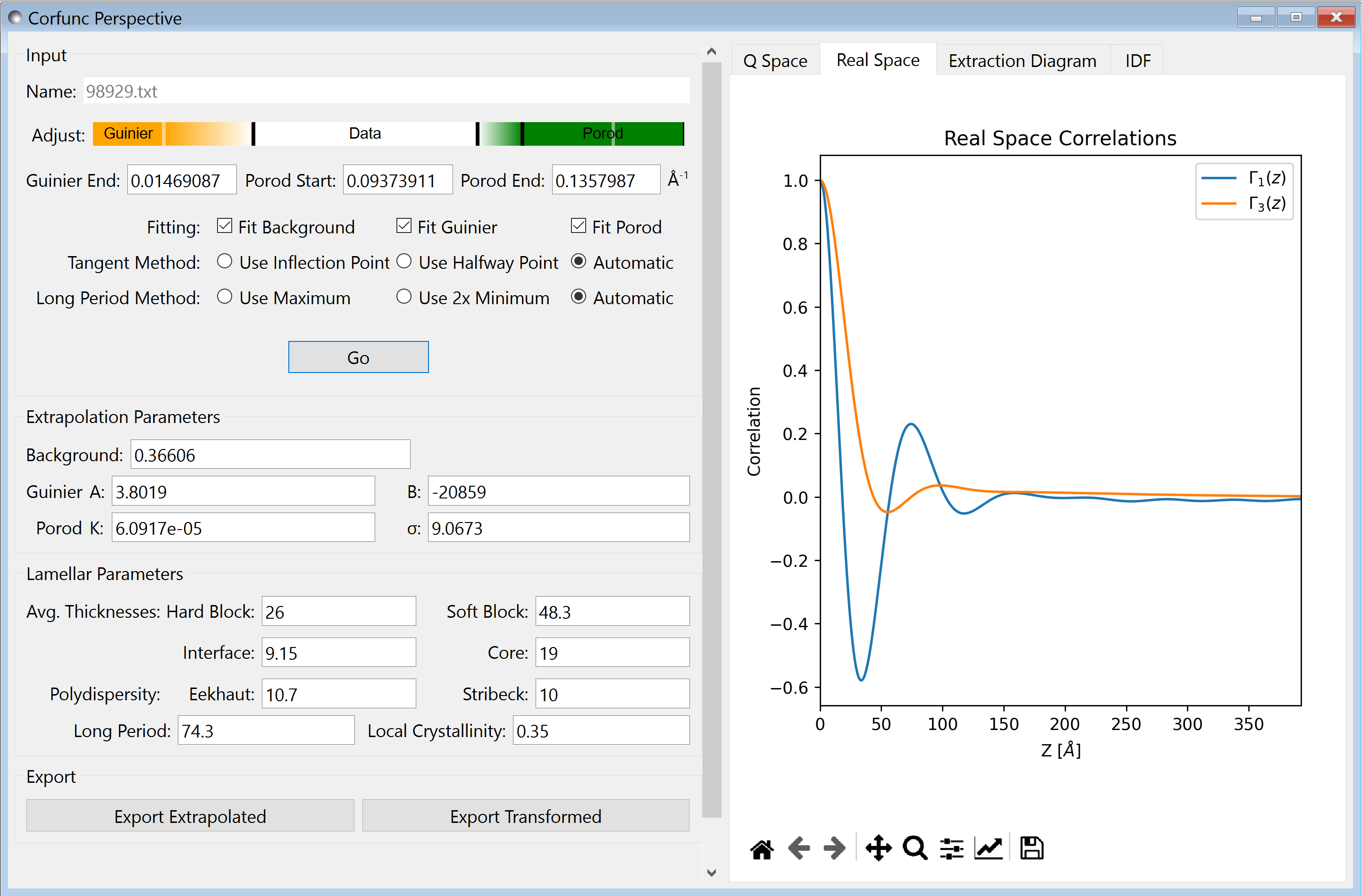
The Real Space tab shows plots of \(\Gamma_1\) and \(\Gamma_3\)
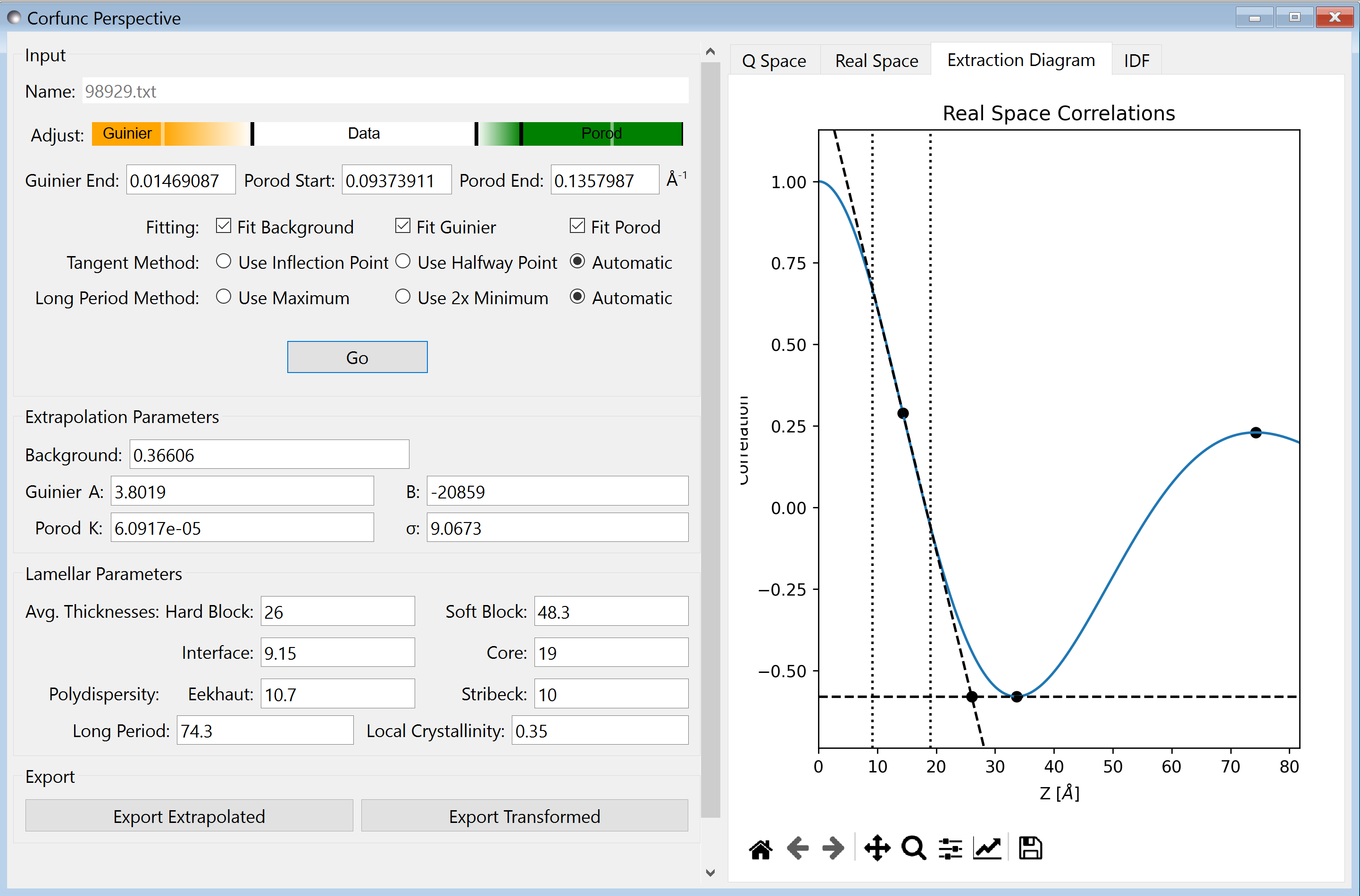
To check the extrapolation parameters, a diagram shows the geometric construction used to derive them in the Extraction Diagram tab.
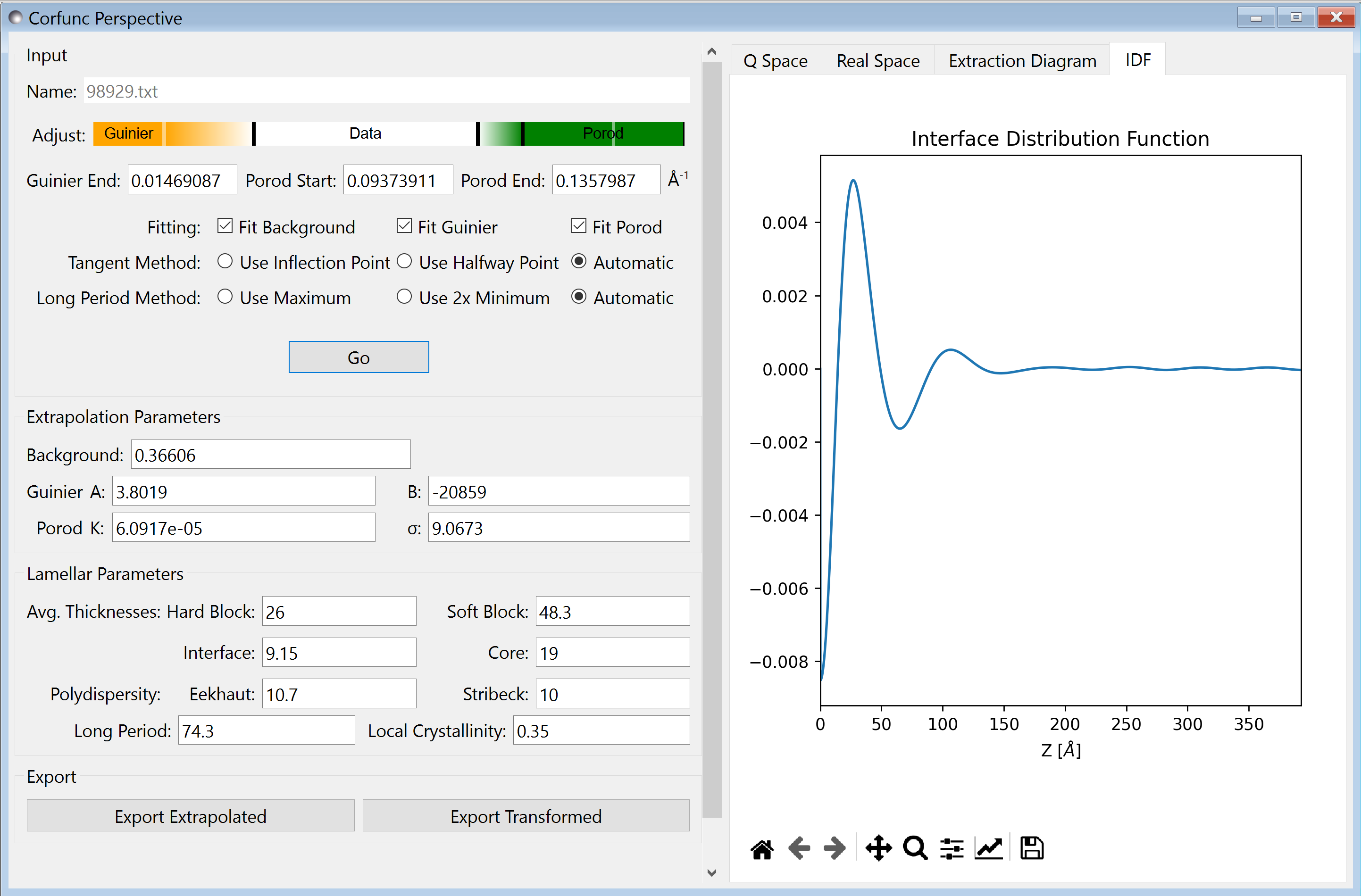
Finally, you can see the interface distribution function in the IDF tab
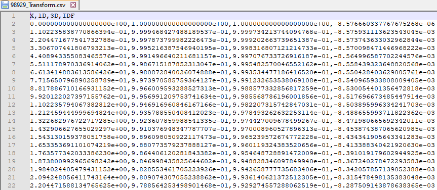
The export buttons allow you to produce CSV files containing either the extrapolated Q-space data, or the transformed data.
The structure of the transformed data file is shown below (note that as this is a 4 column .csv file, SasView will interpret this as a \(I(q)\) vs \(q\) curve if you try to load it from the main SasView window).
Note
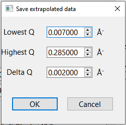
If Export Extrapolated is selected a dialog box will appear in which the bounds and binning of the extrapolated data can be selected. This is pre-populated with the values for the experimental data; i.e. using these values would not actually include any extrapolated data!
