Corfunc Technical Documentation

In Brief

The correlation function analysis is performed in 3 steps.

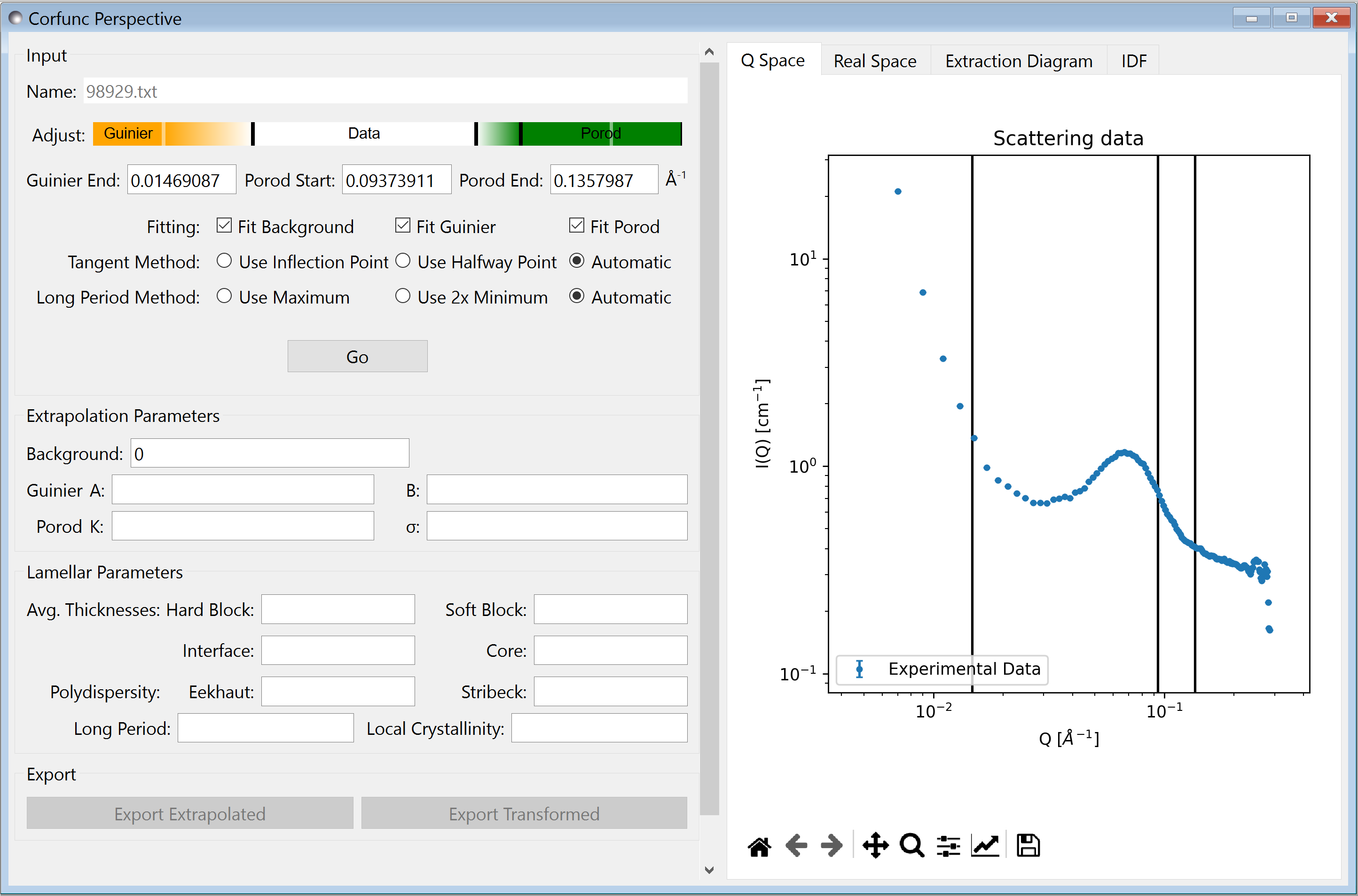
First, the scattering curve is extrapolated to \(Q = 0\) (Guinier) and toward \(Q = \infty\) (Porod), the details of the extrapolation is controlled by the parameters Guinier End, Porod Start and Porod End, which are settable by entering text, or by using the Adjust slider. There is a smooth transition from the data to the extrapolation, start and end refer to the region over which this occurs (see below). Parameters for the extrapolation can manually entered in Extrapolation Parameters and SasView can be told whether to recalcuate the parameters using the Fit Background, Fit Guinier and Fit Porod checkboxes.

Secondly, the data is transformed to obtain the projected correlation functions.

Finally, the transformed data is interpreted in terms of an ideal lamellar morphology

Extrapolation

Small Q

The scattering data is extrapolated to \(q = 0\) by fitting a Guinier function, defined as

\[I(q) = e^{A + Bq^2}\]

to data up to \(q\) value specified by Guinier Start.

This a Gaussian centred at \(q=0\) (we only ever see the positive half). The natural logarithm of the parameter \(A\) is a constant of proportionality equal to the scattering intensity at \(q=0\). The parameter \(B\) describes the width of the function and is related to the size of the scattering object. For example, in systems of dispersed spherical particles it is related to the radius of gyration \(R_g\) by \(B = R_g^2 / 3\).

Note: The Guinier model makes assumptions that do not hold for all systems and so this approximation might not always be accurate. If errors from the Guinier model fit occur, they will manifest as a constant offset in the correlation function, because low \(q\) values correspond to a long periodicity in \(x\). Empirically, however, inaccuracies in the Guinier region have a very low impact on the final analysis, and only some of the lamellar parameters will be affected at all.

Large Q

The data is extrapolated towards \(q = \infty\) by fitting a Porod model, to the region between Porod Start and Porod End. This model is defined by

\[I(q) = K q^{-4} e^{-q^2\sigma^2} + I_{B}\]

Where \(I_B\) is the background intensity, \(K\) is the Porod constant, and \(\sigma\) is a parameter which, in a two phase system, describes the sharpness of the scattering length density profile at the interface between phases.

This model comprises three components, a constant background intensity, the standard Porod law, so

\[I(q) - I_B \propto q^{-4}\]

and a contribution which is attibutable to the sharpness of the boundaries between regions. so

\[I(q) - I_B \propto e^{-q^2\sigma^2}\]

SasView will use this formula to extrapolate to very large \(q\) (100 times the maximum data value). This ensures that the transform used in the next stage does not contain artefacts (i.e. from treating secular data as periodic)

Merging

In the final step before transformation, the experimental and model data are merged together. For the Guinier model, this happens on the region between the start of the experimental data and the value specified by Guinier End. For the Porod model, the merging happens between Porod Start and Porod End.

From	To	Data
0 Start of data Guinier End Porod Start Porod End	Start of data Guinier End Porod Start Porod End 100x end of data	Guinier Model Guinier/Data mix Data Data/Porod mix Porod model

A smooth transition is achieved with sigmoid weighting defined as follows. We start with two input functions, \(f(x)\) on the ‘left’ and \(g(x)\) on the ‘right’, and these are to be smoothed over the range \([a, b]\). We use \(y(x)\) to represent the transition over \([a,b]\). \(y(x)\) is given by the following convex combination

\[y(x) = h(x) g(x) + (1-h(x))f(x)\]

where \(h(x)\) is a weighting between the two, with a value of zero at \(a\) and one at \(b\), defined as

\[h(x) = \frac{1}{1 + \frac{(x-b)^2}{(x-a)^2}}\]

Transformation

Corfunc uses a discrete cosine transform on the extrapolated data in order to calculate the 1D correlation function as:

\[\Gamma _{1}(x) = \frac{1}{Q^{*}} \int_{0}^{\infty }I(q) q^{2} cos(qx) dq\]

where Q^* is the Scattering (also called Porod) Invariant.

The following algorithm is applied:

\[\Gamma(x_k) = 2 \sum_{n=0}^{N-1} x_n \cos{\left[ \frac{\pi}{N} \left(n + \frac{1}{2} \right) k \right] } \text{ for } k = 0, 1, \ldots, N-1, N\]

The 3D correlation function is calculated as:

\[\Gamma _{3}(x) = \frac{1}{Q^{*}} \int_{0}^{\infty}I(q) q^{2} \frac{sin(qx)}{qx} dq\]

Note

It is always advisable to inspect Γ₁(x) and Γ₃(x) for artefacts arising from the extrapolation and transformation processes:

• do they tend to zero as x tends to \(\infty\)?

• do they smoothly curve onto the ordinate at x = 0? (if not check the value of \(\sigma\) is sensible)

• are there ripples at x values corresponding to 2 \(\pi\) over the two q values at which the extrapolated and experimental data are merged?

• are there any artefacts at x values corresponding to 2 \(\pi\) / q_max in the experimental data?

• and lastly, do the significant features/peaks in the correlation functions actually correspond to anticpated spacings in the sample?!!!

Finally, the program calculates the interface distribution function (IDF) g₁(x) as the discrete cosine transform of:

\[q^{4} I(q)\]

The IDF is proportional to the second derivative of Γ₁(x).

Interpretation

Once the correlation functions have been calculated SasView will try and interpret Γ₁(x) in terms of an ideal lamellar morphology as shown below.

It is for the user to decide if this interpretation has any relevance to their system!

The structural parameters extracted are:

• Long Period \(= L_p\)

• Average Hard Block Thickness \(= L_c\)

• Average Core Thickness \(= D_0\)

• Average Interface Thickness \(= D_{tr}\)

• Eekhaut Polydispersity \(= \Gamma_{\text{min}}/\Gamma_{\text{max}}\)

• Stribeck Polydispersity \(= \frac{L_c}{(L_c - L_p)\Gamma_{\text{max}}}\)

• Local Crystallinity \(= L_c/L_p\)

which lead to:

• Average Soft Block Thickness \(= L_p - L_c = L_a\)

• Average Chord Length \(= ((1/L_c) + (1/L_a))^{-1}\)

• Average Crystalline Chord Length \(= \frac{L_a L_c}{\Phi_{\text{c}} (L_c + L_a)}\)

• Non-Ideality \(= \left(\frac{L_p – L_p*}{L_p}\right)^2\)